7 Techniques for Animating Topographic Changes Over Time That Reveal Hidden Patterns

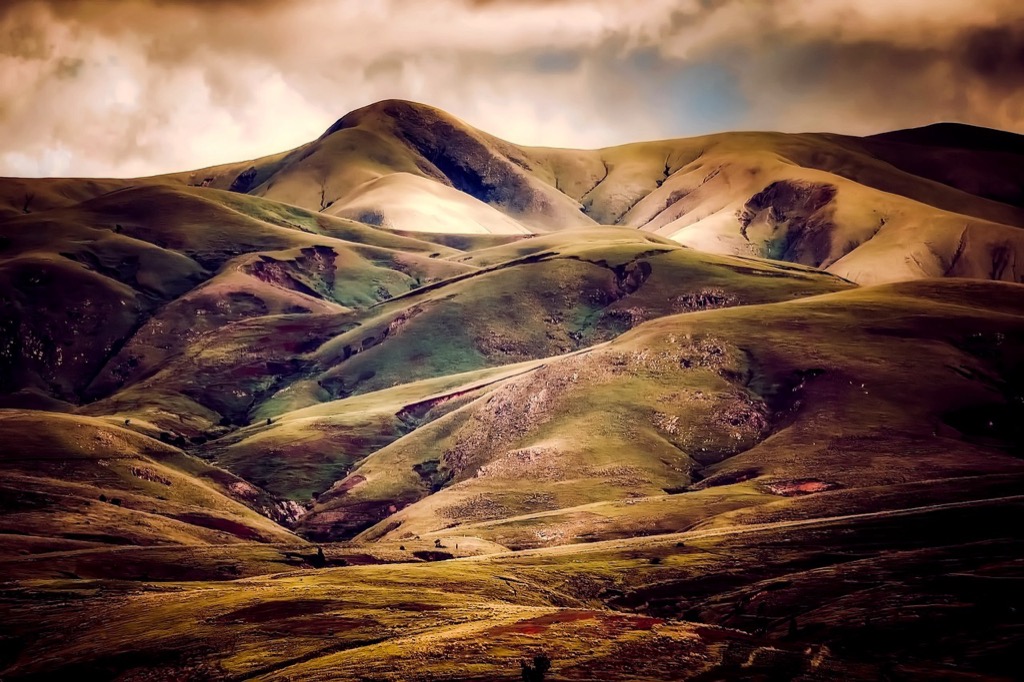
You’re watching glaciers retreat and mountains rise when you view animated topographic maps that compress centuries of geological change into seconds. These powerful visualizations transform static elevation data into compelling stories that reveal how Earth’s surface evolves through natural processes and human activity.

Whether you’re tracking urban development coastal erosion or volcanic activity animated topography helps you communicate complex spatial changes with stunning clarity. The right animation techniques can turn dense geographic data into accessible visual narratives that engage audiences and drive decision-making.

From simple time-lapse sequences to sophisticated morphing algorithms these seven proven methods will help you create professional topographic animations that captivate viewers and convey your message effectively.

Disclosure: As an Amazon Associate, this site earns from qualifying purchases. Thank you!

P.S. check out Udemy’s GIS, Mapping & Remote Sensing courses on sale here…

Technique 1: Time-Lapse Photography and Digital Elevation Model (DEM) Sequencing

Time-lapse photography combined with DEM sequencing creates the foundation for documenting topographic changes with measurable precision. This technique captures both the visual drama and quantitative data needed for professional topographic animations.

Setting Up Ground Control Points for Consistent Reference

Establish permanent markers at stable locations throughout your study area before beginning any temporal analysis. You’ll need at least 6-8 ground control points (GCPs) positioned on bedrock, concrete structures, or other unchanging features to ensure accurate georeferencing across all time periods. Survey these points using high-precision GPS equipment with sub-centimeter accuracy. Document each GCP with detailed photographs and coordinate measurements, creating a reference database that remains consistent throughout your multi-year data collection campaign.

Capturing Multi-Temporal Aerial or Satellite Imagery

Schedule regular aerial surveys at consistent intervals based on your expected rate of change – monthly for rapid erosion studies or annually for gradual geological processes. Use identical flight parameters including altitude, overlap percentages, and camera settings to maintain consistency across temporal datasets. WorldView-3 satellite imagery provides 31cm resolution for large-scale studies, while drone-based photogrammetry offers sub-5cm resolution for detailed local analysis. Capture imagery during similar lighting conditions and seasonal periods to minimize shadows and vegetation differences that could interfere with elevation measurements.

Processing DEM Data for Temporal Analysis

Generate high-resolution DEMs from each temporal dataset using photogrammetric software like Agisoft Metashape or Pix4D, maintaining identical processing parameters across all time periods. Apply consistent filtering algorithms to remove vegetation and structures, creating bare-earth models for accurate topographic comparison. Calculate difference DEMs (DoDs) between sequential time periods, applying statistical significance thresholds of ±10cm vertical accuracy to distinguish real terrain changes from measurement noise. Export your processed elevation datasets in standardized formats like GeoTIFF for seamless integration into animation software.

Technique 2: LiDAR Point Cloud Animation Through Temporal Registration

LiDAR point cloud animation builds upon the precision of laser scanning technology to capture millimeter-level topographic changes across multiple time periods. This technique excels at documenting subtle elevation shifts that traditional photogrammetry might miss.

Acquiring Multi-Date LiDAR Datasets

You’ll need to establish consistent flight parameters across all acquisition dates to ensure temporal compatibility. Maintain identical pulse density specifications (typically 8-12 points per square meter) and flight altitudes between surveys. Schedule flights during similar atmospheric conditions and vegetation states to minimize seasonal variations. Coordinate with LiDAR service providers to use the same sensor specifications and calibration standards. Document ground control points before each flight mission to verify georeferencing accuracy throughout your temporal sequence.

Aligning Point Clouds Using Registration Algorithms

You should apply Iterative Closest Point (ICP) algorithms to align overlapping point clouds from different time periods. Focus registration on stable terrain features like bedrock outcrops or permanent structures that haven’t changed between surveys. Use CloudCompare or LAStools to perform fine-scale alignment adjustments after initial georeferencing. Apply M3C2 (Multiscale Model to Model Cloud Comparison) algorithms to calculate precise distance measurements between temporal datasets. Validate registration accuracy by measuring unchanged reference surfaces that should show zero elevation difference.

Creating Smooth Transitions Between Time Periods

You can generate interpolated point clouds between actual survey dates using temporal morphing algorithms. Create intermediate frames by blending XYZ coordinates proportionally across your timeline to produce fluid animation sequences. Apply Gaussian smoothing filters to eliminate registration artifacts and noise between temporal transitions. Set consistent point cloud density across all animation frames to prevent visual flickering during playback. Export your temporal sequence as standardized LAS files for integration with visualization software like Potree or CloudCompare’s animation tools.

Technique 3: Contour Line Morphing and Interpolation Methods

Contour line morphing transforms historical elevation data into smooth temporal animations by interpolating between different time periods. This technique proves especially valuable when working with historical survey data or scanned topographic maps where traditional DEM methods aren’t feasible.

Extracting Contour Lines from Historical Maps

You’ll need to digitize contour lines from scanned historical maps using semi-automated vectorization tools like ArcGIS’s ArcScan or QGIS’s raster tracing plugins. Start by georeferencing your historical maps to a consistent coordinate system, then apply edge detection algorithms to identify contour boundaries. Manual cleanup remains essential – automated extraction typically achieves 70-80% accuracy, requiring careful review of elevation labels and contour continuity. Store extracted contours as polyline features with elevation attributes for seamless integration into morphing workflows.

Applying Morphing Algorithms to Transition Between Contours

Morphing algorithms create smooth transitions by calculating intermediate contour positions between temporal datasets. The Thin Plate Spline (TPS) interpolation method works best for gradual topographic changes, while Inverse Distance Weighting (IDW) handles abrupt elevation shifts more effectively. Configure your morphing parameters to generate 10-15 intermediate frames per time interval for fluid animation playback. Popular tools include Blender’s shape keys for 3D morphing or custom Python scripts using NumPy’s interpolation functions for precise control over temporal transitions.

Optimizing Interpolation Parameters for Realistic Movement

Fine-tune your interpolation settings to match the geological processes you’re documenting. Set power parameters between 1.5-2.5 for IDW interpolation when modeling gradual erosion, while using lower values (0.8-1.2) for sudden landslide events. Adjust search radius to 3-5 times your contour interval for optimal smoothing without losing detail. Test different temporal weighting functions – linear interpolation works for consistent processes, while exponential curves better represent accelerating changes like glacier retreat or urban development impacts.

Technique 4: 3D Mesh Deformation Using Keyframe Animation

3D mesh deformation transforms static terrain into dynamic visualizations by manipulating vertex positions through keyframe animation. This technique provides precise control over topographic changes while maintaining mesh topology consistency.

Building Base 3D Terrain Meshes from Topographic Data

Convert your elevation data into triangulated irregular networks (TINs) using software like ArcGIS Pro or QGIS. Generate meshes with consistent vertex density across all temporal datasets to ensure smooth deformation. Apply Delaunay triangulation algorithms to create optimal triangle distributions that preserve terrain features. Export base meshes in standardized formats like OBJ or PLY for compatibility with animation software such as Blender or Maya.

Setting Keyframes for Major Topographic Changes

Define temporal keyframes at critical change intervals based on your dataset’s resolution and the geological processes you’re documenting. Position keyframes at 10-20% intervals of your total timeline for gradual changes like erosion, or concentrate them around rapid events like landslides. Configure vertex positions for each keyframe state by mapping elevation differences to Z-axis displacement values. Store keyframe data as vertex animation caches to maintain rendering performance during playback.

Implementing Smooth Mesh Deformation Between States

Apply interpolation algorithms like linear or Bézier curves to create fluid transitions between keyframes. Use vertex-based morphing techniques that calculate intermediate positions for each mesh point during animation frames. Configure easing functions such as ease-in-out curves to simulate realistic geological movement patterns. Implement collision detection to prevent mesh self-intersection during extreme deformation sequences, particularly when animating dramatic elevation changes exceeding 50 meters.

Technique 5: Particle System Simulation for Erosion and Sediment Transport

Particle system simulation recreates the complex dynamics of water flow and sediment movement through physics-based calculations. This technique transforms static topographic data into realistic erosion animations by modeling individual particles as they interact with terrain surfaces over time.

Modeling Water Flow Patterns and Erosion Processes

Flow simulation algorithms calculate water movement across digital terrain models using hydraulic principles and surface roughness coefficients. You’ll implement shallow water equations to determine flow velocity and direction based on elevation gradients and Manning’s roughness values. Erosion rate calculations integrate flow velocity with soil erodibility factors to determine material removal at each terrain point. Configure particle spawn rates between 100-500 particles per simulation timestep depending on watershed size and computational resources available.

Simulating Sediment Movement and Deposition

Sediment transport modeling tracks individual soil particles as they move downstream according to flow velocity and particle size distributions. You’ll apply Hjulström-Sundborg curves to determine when particles become suspended transported or deposited based on current velocity thresholds. Deposition algorithms calculate settling locations using particle density and flow turbulence parameters. Set carrying capacity limits between 0.1-2.0 kg/m³ depending on soil type with sandy soils requiring lower thresholds than clay-rich materials.

Integrating Physics-Based Calculations for Realistic Results

Physics integration systems combine gravitational forces fluid dynamics and particle collision detection to create believable sediment behavior patterns. You’ll implement Verlet integration methods with timesteps between 0.01-0.1 seconds to maintain numerical stability during complex interactions. Calibration procedures validate simulation results against field measurements or historical erosion data using statistical correlation coefficients above 0.75. Apply adaptive mesh refinement techniques to concentrate computational resources on areas experiencing rapid topographic change while maintaining overall animation performance.

Technique 6: Height Field Animation Through Mathematical Functions

Mathematical functions provide precise control over topographic animation by treating elevation data as continuous surfaces that can be manipulated algorithmically. This technique excels when you need smooth, predictable terrain changes based on scientific models.

Converting Topographic Data to Height Field Formats

Transform your DEM data into height field arrays using raster processing software like GDAL or ArcGIS Spatial Analyst. Export elevation values as normalized grayscale images where pixel intensity represents elevation magnitude. You’ll need consistent spatial resolution across all temporal datasets—typically 1-meter or 5-meter cell sizes work best for detailed animations. Store height fields as 32-bit floating-point TIFF files to preserve elevation precision during mathematical operations.

Applying Mathematical Functions for Gradual Elevation Changes

Apply sinusoidal functions for cyclical changes like seasonal frost heave or polynomial interpolation for gradual processes like subsidence. Use exponential decay functions to model erosion rates: h(t) = h₀ * e^(-kt) where k represents erosion constant. Linear interpolation works well for steady uplift: h(t) = h₀ + (rate * time). Combine multiple functions using weighted averages to simulate complex geological processes affecting different terrain zones simultaneously.

Controlling Animation Speed and Timing Parameters

Set frame rates between 24-30 fps for smooth playback while maintaining reasonable file sizes. Use temporal scaling factors to compress geological time—apply logarithmic time steps for long-term processes spanning millennia. Control interpolation timing with easing functions: ease-in for accelerating processes, ease-out for decelerating changes. You can adjust animation duration by modifying the time parameter range in your mathematical functions, typically spanning 100-500 frames for effective visualization.

Technique 7: Multi-Layer Composite Animation Using Geographic Information Systems (GIS)

Multi-layer composite animation transforms complex topographic changes into cohesive visualizations by integrating diverse temporal datasets within GIS environments. This technique leverages the analytical power of spatial databases to synchronize multiple geographic elements across extended time periods.

Combining Multiple Data Sources and Time Periods

Integrate diverse temporal datasets by establishing a master timeline that accommodates varying data collection frequencies. You’ll combine satellite imagery intervals (monthly), LiDAR surveys (annual), and historical maps (decadal) within a unified coordinate system. Use ArcGIS Pro’s Time Slider or QGIS Temporal Controller to manage multi-resolution temporal data effectively. Standardize all datasets to consistent projections and cell sizes before temporal integration. Apply temporal interpolation algorithms to fill data gaps between acquisition periods.

Creating Layered Animations with Transparency Effects

Build visual depth through strategic transparency layering that reveals subsurface processes and historical contexts. Set base terrain layers at 100% opacity while applying 30-70% transparency to overlying temporal elements like vegetation change or urban development. Use graduated transparency values to emphasize recent changes over historical baselines. Implement blending modes such as “Multiply” for geological layers and “Screen” for highlighting effects. Control layer visibility through time-based rules that automatically adjust transparency values during animation playback.

Synchronizing Different Geographic Elements and Features

Coordinate temporal elements by establishing synchronized keyframes that align hydrological, geological, and anthropogenic changes. Configure master timing controls that govern all animated layers simultaneously while allowing individual layer offset adjustments. Use temporal joins to link attribute tables across different time periods for consistent feature symbolization. Apply consistent animation curves (linear, ease-in, ease-out) across all geographic elements to maintain visual cohesion. Validate synchronization through preview rendering that checks for temporal misalignment between interacting features.

Conclusion

These seven animation techniques give you the power to transform static topographic data into compelling visual stories. Whether you’re documenting glacial retreat or urban expansion your choice of method depends on your specific project requirements and available resources.

Success lies in matching the right technique to your data type and audience needs. LiDAR point clouds work best for precision documentation while particle systems excel at showing dynamic processes like erosion.

Remember that effective topographic animation combines technical accuracy with visual appeal. Start with one technique that fits your current skill level then gradually expand your toolkit as you gain experience.

Your animated topographic visualizations can become powerful tools for education research and decision-making. The key is consistent practice and willingness to experiment with different approaches until you find what works best for your unique projects.

Frequently Asked Questions

What are animated topographic maps and why are they useful?

Animated topographic maps are visualizations that show how landscapes change over time, illustrating processes like glacier retreat, mountain formation, urban development, and coastal erosion. They’re highly effective for communicating complex spatial changes in an engaging, easy-to-understand format that enhances decision-making and captivates audiences with both visual appeal and quantitative data.

What is time-lapse photography combined with DEM sequencing?

This technique combines dramatic visual imagery with quantitative elevation data to document topographic changes. It involves establishing ground control points (GCPs) for accurate georeferencing and capturing multi-temporal aerial or satellite imagery at consistent intervals. This method provides both compelling visuals and precise measurements of landscape transformation over time.

How does LiDAR point cloud animation work?

LiDAR point cloud animation uses laser scanning technology to capture millimeter-level topographic changes across multiple time periods. It requires consistent flight parameters and atmospheric conditions to ensure accuracy. This technique excels at detecting subtle elevation changes and creating highly detailed animations of landscape evolution.

What is contour line morphing and interpolation?

This method transforms historical elevation data into smooth temporal animations by digitizing contour lines from maps and applying morphing algorithms. The process creates realistic transitions between different time periods, allowing viewers to see how elevation patterns have changed gradually over time through fluid, continuous animation.

How does 3D mesh deformation with keyframe animation work?

This technique creates dynamic visualizations by manipulating vertex positions in 3D meshes while maintaining consistent mesh topology. It uses keyframe animation principles to show landscape changes, allowing for precise control over how terrain features evolve and providing smooth transitions between different topographic states.

What is particle system simulation for erosion visualization?

Particle system simulation recreates the dynamics of water flow and sediment transport through physics-based calculations. This technique visualizes erosion processes by simulating how particles move across terrain, showing sediment transport patterns and helping viewers understand the physical processes that shape landscapes over time.

What is multi-layer composite animation using GIS?

This technique integrates diverse temporal datasets within Geographic Information Systems to create cohesive visualizations. It combines satellite imagery, LiDAR surveys, and historical maps in a unified coordinate system, using master timelines, transparency effects, and synchronized geographic elements to maintain visual cohesion across different data sources.